Load/performance testing a Rails application with ApacheBench

Published by Martin Kleppmann on 27 Oct 2008.

Just over 3 days until Bid for Wine goes online! It’s great to see this massive project, which I’ve blogged about before, finally complete. We will launch on Friday 31 October, the first lots for sale are already lined up (including a remarkable bottle – a unique item from a private bottling of the famous Guigal Family, and probably the only bottle of its kind on the open market!), some big wine magazines are going to be reporting, and everybody is getting very excited.

The application is deployed to the servers (we are running on Engine Yard), the DNS is updated, the load balancers are configured, the holding page and contact form are already getting a fair bit of traffic, everything seems ready. We just need to flick a switch and users will start hitting the site.

Hold on. How do we know that the site won’t just immediately collapse under the load of (hopefully many) visitors hitting the site at the same time? The last thing we would want to do is to put them off by going down straight after launch. Some load testing is in order.

That said, we don’t want to spend much time and money on it either. It doesn’t need to be an enterprise-grade solution. All I want to do is check that we won’t fall over and die if we get lots of nice people coming to visit us.

I’m aware that with load tests, you need to be quite careful that you end up actually testing the server; it can happen easily that the bottleneck is actually somewhere on the client’s side. So part of this experiment was actually to test the load testing tool, not just the target application!

The tool I used here is ApacheBench; there are others, like http_load and siege, which I may try another time. I booted up an EC2 instance specifically for running ApacheBench, to provide a clean ‘laboratory’ environment without processes contending for CPU and I/O. I ran a variety of tests using different URLs, sending cookies (to simulate a logged-in user), with and without keep-alive etc. These parameters all changed the results a bit, but the general shape was the same, so here’s some data for one particular page (the auction listing view).

ApacheBench lets you set the level of concurrency, i.e. the number of connections it tries to make to the server at the same time. We have two EngineYard production slices (virtual machines), each running three Mongrels (the single-threaded server daemons which run the application), so I expected that we should be able to handle six concurrent connections without any queueing of requests.

The first graph is for a test with four concurrent connections, i.e. the server should be pretty relaxed. It shows which proportion of pages were served in less than a particular time (i.e. the percentiles). The graph is generated from timings of 10,000 page views.

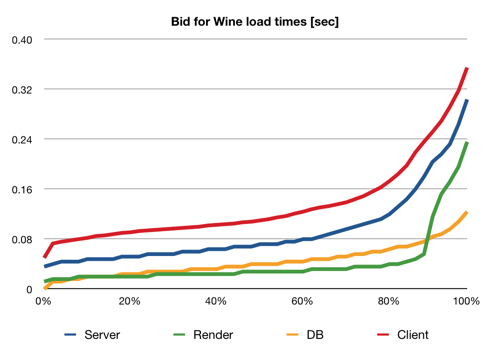
How to read this graph: e.g. see that the red line crosses 0.16 seconds at about 80%; that means that the client (ApacheBench) reported that 80% of requests were served in 0.16 seconds or less. The highest point at 100% is the longest time which it ever took in the test.

I measured four quantities: the time per page view reported by ApacheBench (the client), the total time per page view reported by the server, and the values for rendering time and database time reported by the server. (The blue line is the sum of the green and the orange lines.) I would call this pretty well-behaved: 84% of page requests are received by the client within 200 milliseconds, and 95% within 300ms; rendering time is quite variable while database time hardly ever exceeds 100ms. And the client times are just a constant amount above the server times, to account for the fact that the request and response have to go across a network, through a proxy/load balancer etc.

Each of those page views involves about 11 SQL queries and 10 partials being rendered; we can’t get much below that, since the page content is fairly complex. My guess is that you can’t do much better than these timings with Ruby on Rails out of the box; at the end of the day, it is a pretty slow platform. (I’m not saying that other languages/frameworks are any better – most likely, they are not.) When we find that this site needs to scale further, we will simply have to add more mongrels, database read slaves, and plenty of memcached to the system.

By the way, in this test the 1-minute load average reported by the Linux kernel reached a maximum of 1.6 – not very much at all.

Now, what happens when we hit the site harder? In the next test I increased the concurrency parameter to 16, more than twice the number of mongrels. Now I would expect all mongrels to be busy all the time (saturated with requests), and response times to go up. And this is the graph we get:

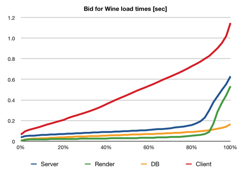
Ignore the red one for now. The shape of the three server-side curves is still pretty much the same as before, and overall they are taking 50% to 100% longer to respond compared to the test above. That is simply because the CPU is now fully occupied with all three mongrels, whereas previously there might only be one or two mongrels wanting CPU at the same time. When I ran further tests, increasing concurrency of the client to 64 (more than ten times the number of mongrels), these server curves stayed exactly the same, and server-side times didn’t increase any further. This is good news: although the server is overloaded, this doesn’t cause any loss of throughput (which might be the case if there were inefficiencies).

For a saturated server, the kernel load average was between about 3.0 and 4.0, no matter how many concurrent clients there were. This makes sense, since the load is determined by the length of the scheduler’s run queue, and if you only have 3 server processes (mongrels) plus a few of background housekeeping processes with small requirements, there’s no reason why it should go any higher.

The combined throughput of the mongrels in this test, and in those with higher concurrency, was pretty constant at 33 requests per second. Since that is across 2 CPUs, we must be taking 60ms of CPU time per request, or an average of 180ms wall-clock time (1 CPU is shared between 3 mongrels). The average request time (DB + Render) reported by the server is 164ms, so we have only 10% overhead somewhere which is not being accounted for. Nice to see that the numbers add up quite well. :-)

Now turn your attention to the red line, which is now completely different from before. There are still some page views which happen very quickly, but some are taking up to a whole second. What is happening here is that requests are getting queued up – if they are lucky, the queue is empty and they get served right away, but if it’s their bad day, they might have to wait in line after several other requests until they finally get to talk to a mongrel. The mongrels work at the same pace, no matter how long the queue is (think post office workers), so obviously waiting times will increase the more people/requests try to get in the door at the same time.

With 16 concurrent clients, the median response time was 0.45 seconds, and 99% of requests were served within 1.3 seconds. However, with 64 concurrent clients, the median was 1.8 seconds and the 99% percentile was a whopping 6.2 seconds. (This is the point where users get rather impatient.) I’m not sure exactly what the relationship between concurrency and waiting time is; maybe with some more experiments and some theory I can work it out. (I took a course on queueing theory at university, which covers exactly this kind of system, but I can’t remember much of it. If I have time I’ll dig it out again and see how I might be able to model traffic to a web application with lots of nice maths…)

The thing which struck me in this graph is quite how straight that red line is; I had expected the response times to be less widely spread. This prompted me to have a look at the actual distribution/histogram of response times as reported by the client.

Another thing I wanted to check was how good ApacheBench’s concurrency setting actually was – how could I trust that it really keeps the server as busy as it claims to? And maybe it makes requests in certain regular patterns which might skew the results. So I ran the following 3 tests in a side-by-side comparison:

1. One ApacheBench process set to make 64 concurrent requests, running on an EC2 instance, no keep-alive, making 10,000 requests.
2. Four ApacheBench processes, each set to make 16 concurrent requests, running on the same EC2 instance, no keep-alive, each making 2,500 requests.
3. Four ApacheBench processes, each set to make 16 concurrent requests, each running on its own EC2 instance, no keep-alive, each making 2,500 requests.

The server-side statistics for the three tests, including the total throughput, were identical. However, interestingly, there was a noticeable difference between the distribution of response times reported by ApacheBench in the three cases. I have plotted them below:

(This diagram is what you get if you flip the one above by a diagonal axis and then differentiate the function by response time. Note also that the colours now have a different meaning.)

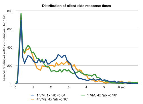
I don’t quite know yet what to make of this. Ok, the behaviour doesn’t differ too drastically, so if you just want a rough idea of the performance of your application, it seems like ApacheBench’s concurrency option is perfectly fine. I am just a bit intrigued by the differences.

The green line is most like what I expected, because it most resembles an exponential distribution, which is what queueing theory predicts in many cases. Interestingly, this is the setup in which the four ApacheBench processes are most likely to get in each other’s way, contending for I/O on the EC2 instance – maybe this causes some jitter, blurring an otherwise regular pattern. In the two cases with one ApacheBench process per machine (blue and yellow lines) the distribution is more flat between about 1 and 3 seconds response time; in particular, the blue and yellow setup are noticeably more likely to see 2-3 second response times than the green setup.

If anybody has ideas on how to interpret this, please let me know. I should probably also repeat those experiments with a larger sample size and work out if the differences are actually statistically significant, but I don’t have time for that at the moment.

SCRIPTS

In order to produce these statistics, I wrote a few simple shell scripts to gather and process the data. I’ll put them here in case somebody finds them useful (and so that I can find them again when I need them next time!).

First I have two scripts which run on the servers with the mongrels. In our setup, each virtual machine has its own logfile, so the scripts need to be run on each virtual machine. They select the portion of the logfile which was written during the duration of the test, and also log load averages from the kernel. Set an environment variable like export LOGFILE=/path/to/my/production.log before running these scripts. The first is called before-test.sh and should be run before the test starts:

#!/bin/sh
if [ ! -f "$LOGFILE" ]; then echo "LOGFILE not found"; exit 1; fi
echo "time,1min,5min,10min,running,procs,lastproc" > /tmp/loadavg.csv
( while true; do

ts=`date '+%Y%m%d%H%M%S'`
load="`cat /proc/loadavg | tr ' /' ','`"
echo "$ts,$load" >> /tmp/loadavg.csv
sleep 1
done ) &
echo $! > /tmp/loadavg.pid
wc -l $LOGFILE | awk '{print $1}' > /tmp/skip_log_lines

And after-test.sh should be run when the test has ended:

#!/bin/sh
kill `cat /tmp/loadavg.pid`
echo "total,render,db,url" > /tmp/requests.csv
skip=`cat /tmp/skip_log_lines`
tail -n +`expr $skip + 1` $LOGFILE | grep
'^Completed in' | \\
awk '{print $3 "," $8 "," $12 "," $17}' >> /tmp/requests.csv
rm -f /tmp/loadavg.pid /tmp/skip_log_lines

As you can see, it filters the processing times reported by the server out of the logfile and formats them as CSV for post-processing in your favourite spreadsheet application.

To execute the test (potentially with several processes at the same time), I ran something like the following on an EC2 instance:

apt-get update
apt-get -y dist-upgrade
apt-get -y install
apache2-utils
mkdir loadtest
cd loadtest
TESTS="list1 list2 list3 list4"
COOKIE="-C _session_id=12345678901234567890"
HOST="http://staging.example.com/"
AB="ab -n 10000 -c 16" # 10,000 requests, concurrency 16 per process
$AB -g list1.log $COOKIE "${HOST}/path/to/test" &
$AB -g list2.log $COOKIE "${HOST}/path/to/test" &
$AB -g list3.log $COOKIE "${HOST}/path/to/test" &
$AB -g list4.log $COOKIE "${HOST}/path/to/test" &
wait
for test in $TESTS; do
awk -F '\' "{print \\$4 \\",\\" \\$5 \\",\\" \\$6 \\",$test\\"}" < $test.log | tail -n +2 > $test
done
echo "dtime,ttime,wait,test" > bench.csv
cat $TESTS >> bench.csv

Then copying and aggregating all the logs onto my machine for making pretty graphs:

TEST=test7
CLIENTS="ec2-75-101-204-213"
KEYFILE="path/to/private/key/file/for/ec2/instance"
for host in prod1 prod2; do
for file in loadavg requests; do
scp "ey-$host:/tmp/$file.csv" "$file-$host.csv"
done
done
for client in $CLIENTS; do
scp -i $KEYFILE root@$client.compute-1.amazonaws.com:loadtest/bench.csv client-$client.csv
done
mkdir $TEST
paste -d ',' loadavg-prod1.csv loadavg-prod2.csv > $TEST/loadavg.csv
cat requests-prod\[12\].csv > $TEST/requests.csv
cat client*.csv > $TEST/clients.csv
mv loadavg-prod\[12\].csv requests-prod\[12\].csv client*.csv $TEST

Obviously these scripts are still pretty rough around the edges, but they did the job of being simple and telling me what I wanted to know.