Using Bloom filters to efficiently synchronise hash graphs

Published by Martin Kleppmann on 02 Dec 2020.

This blog post uses MathJax to render mathematics. You need JavaScript enabled for MathJax to work.

In some recent research, Heidi and I needed to solve the following problem. Say you want to sync a hash graph, such as a Git repository, between two nodes. In Git, each commit is identified by its hash, and a commit may include the hashes of predecessor commits (a commit may include more than one hash if it’s a merge commit). We want to figure out the minimal set of commits that the two nodes need to send to each other in order to make their graphs the same.

You might wonder: isn’t this a solved problem? Git has to do this every time you do git pull or git push! You’re right, and some cases are easy, but other cases are a bit trickier. What’s more, the algorithm used by Git is not particularly well-documented, and in any case we think that we can do better.

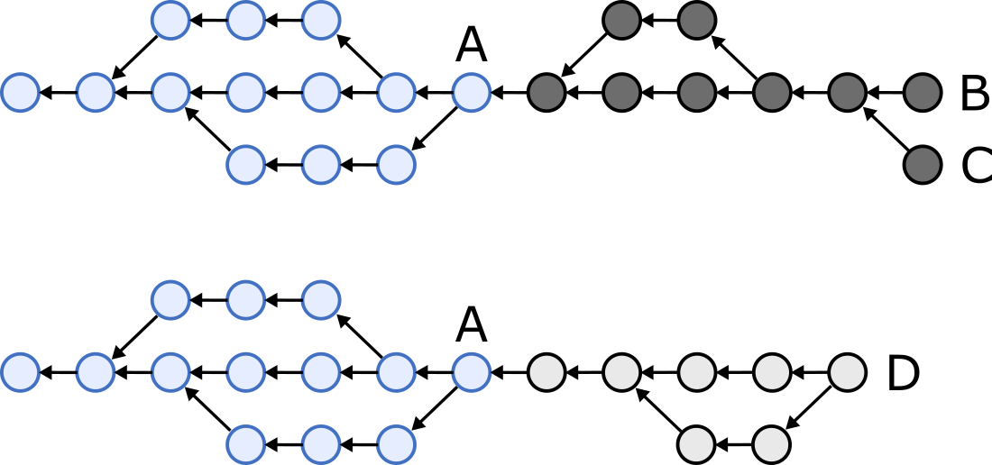
For example, say we have two nodes, and each has one of the following two hash graphs (circles are commits, arrows indicate one commit referencing the hash of another). The blue part (commit A and those to the left of it) is shared between the two graphs, while the dark grey and light grey parts exist in only one of the two graphs.

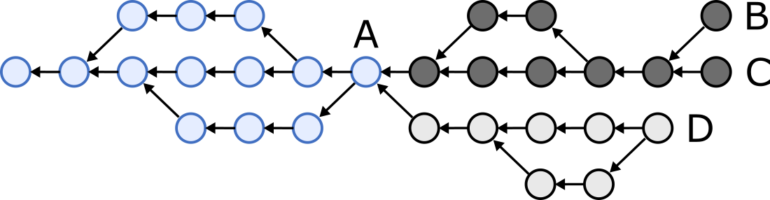
We want to reconcile the two nodes’ states so that one node sends all of the dark-grey-coloured commits, the other sends all of the light-grey-coloured commits, and both end up with the following graph:

How do we efficiently figure out which commits the two nodes need to send to each other?

Traversing the graph

First, some terminology. Let’s say commit A is a predecessor of commit B if B references the hash of A, or if there is some chain of hash references from B leading to A. If A is a predecessor of B, then B is a successor of A. Finally, define the heads of the graph to be those commits that have no successors. In the example above, the heads are B, C, and D. (This is slightly different from how Git defines HEAD.)

The reconciliation algorithm is easy if it’s a “fast-forward” situation: that is, if one node’s heads are commits that the other node already has. In that case, one node sends the other the hashes of its heads, and the other node replies with all commits that are successors of the first node’s heads. However, the situation is tricker in the example above, where one node’s heads B and C are unknown to the other node, and likewise head D is unknown to the first node.

In order to reconcile the two graphs, we want to figure out which commits are the latest common predecessors of both graphs’ heads (also known as common ancestors, marked A in the example), and then the nodes can send each other all commits that are successors of the common predecessors.

As a first attempt, we can try this: the two nodes send each other their heads; if those contain any unknown predecessor hashes, they request those, and repeat until all hashes resolve to known commits. Thus, the nodes gradually work their way from the heads towards the common predecessors. This works, but it is slow if your graph contains long chains of commits, since the number of round trips required equals the length of the longest path from a head to a common predecessor.

The “smart” transfer protocol used by Git essentially works like this, except that it sends 32 hashes at a time in order to reduce the number of round trips. Why 32? Who knows. It’s a trade-off: send more hashes to reduce the number of round trips, but each request/response is bigger. Presumably they decided that 32 was a reasonable compromise between latency and bandwidth.

Recent versions of Git also support an experimental “skipping” algorithm, which can be enabled using the fetch.negotiationAlgorithm config option. Rather than moving forward by a fixed number of predecessors in each round trip, this algorithm allows some commits to be skipped, so that it reaches the common predecessors faster. The skip size grows similarly to the Fibonacci sequence (i.e. exponentially) with each round trip. This reduces the number of round trips to \(O(\log n)\), but you can end up overshooting the common predecessors, and thus the protocol may end up unnecessarily transmitting commits that the other node already has.

Bloom filters to the rescue

In our new paper draft, which we are making available on arXiv today, Heidi and I propose a different algorithm for performing this kind of reconciliation. It is quite simple if you know how Bloom filters work.

In addition to sending the hashes of their heads, each node constructs a Bloom filter containing the hashes of the commits that it knows about. In our prototype, we allocate 10 bits (1.25 bytes) per commit. This number can be adjusted, but note that it is a lot more compact than sending the full 20-byte (for SHA-1, used by Git) or 32-byte (for SHA-256, which is more secure) hash for each commit. Moreover, we keep track of the heads from the last time we reconciled our state with a particular node, and then the Bloom filter only needs to include commits that were added since the last reconciliation.

When a node receives such a Bloom filter, it checks its own commit hashes to see whether they appear in the filter. Any commits whose hash does not appear in the Bloom filter, and its successors, can immediately be sent to the other node, since we can be sure that the other node does not know about those commits. For any commits whose hash does appear in the Bloom filter, it is likely that the other node knows about that commit, but due to false positives it is possible that the other node actually does not know about those commits.

After receiving all the commits that did not appear in the Bloom filter, we check whether we know all of their predecessor hashes. If any are missing, we request them in a separate round trip using the same graph traversal algorithm as before. Due to the way the false positive probabilities work, the probability of requiring n round trips decreases exponentially as n grows. For example, you might have a 1% chance of requiring two round trips, a 0.01% chance of requiring three round trips, a 0.0001% chance of requiring four round trips, and so on. Almost all reconciliations complete in one round trip.

Unlike the skipping algorithm used by Git, our algorithm never unnecessarily sends any commits that the other side already has, and the Bloom filters are very compact, even for large commit histories.

Practical relevance

In the paper we also prove that this algorithm allows nodes to sync their state even in the presence of arbitrarily many malicious nodes, making it immune to Sybil attacks. We then go on to prove a theorem that shows which types of applications can and cannot be implemented in this Sybil-immune way, without requiring any Sybil countermeasures such as proof-of-work or the centralised control of permissioned blockchains.

All of this is directly relevant for local-first peer-to-peer applications in which apps running on different devices need to sync up their state without necessarily trusting each other or relying on any trusted servers. I assume it’s also relevant for blockchains that use hash graphs, but I don’t know much about them. So, syncing a Git commit history is just one of many possible use cases – I just used it because most developers will be at least roughly familiar with it!

The details of the algorithm and the theorems are in the paper, so I won’t repeat them here. Instead, I will briefly mention a few interesting things that didn’t make it into the paper.

Why Bloom filters?

One thing you might be wondering: rather than creating a Bloom filters with 10 bits per commit, can we not just truncate the commit hashes to 10 bits and send those instead? That would use the same amount of network bandwidth, and intuitively it may seem like it should be equivalent.

However, that is not the case: Bloom filters perform vastly better than truncated hashes. I will use a small amount of probability theory to explain why.

Say we have a hash graph containing \(n\) distinct items, and we want to use \(b\) bits per item (so the total size of the data structure is \(m=bn\) bits). If we are using truncated hashes, there are \(2^b\) possible values for each \(b\)-bit hash. Thus, given two independently chosen, uniformly distributed hashes, the probability that they are the same is \(2^{-b}\).

If we have \(n\) uniformly distributed hashes, the probability that they are all different from a given \(b\)-bit hash is \((1-2^{-b})^n\). The false positive probability is therefore the probability that a given \(b\)-bit hash equals one or more of the \(n\) hashes:

\[ P(\text{false positive in truncated hashes}) = 1 - (1 - 2^{-b})^n \]

On the other hand, with a Bloom filter, we start out with all \(m\) bits set to zero, and then for each item, we set \(k\) bits to one. After one uniformly distributed bit-setting operation, the probability that a given bit is zero is \(1 - 1/m\). Thus, after \(kn\) bit-setting operations, the probability that a given bit is still zero is \((1 - 1/m)^{kn}\).

A Bloom filter has a false positive when we check \(k\) bits for some item and they are all one, even though that item was not in the set. The probability of this happening is

\[ P(\text{false positive in Bloom filter}) = (1 - (1 - 1/m)^{kn})^k \]

It’s not obvious from those expressions which of the two is better, so I plotted the false positive probabilities of truncated hashes and Bloom filters for varying numbers of items \(n\), and with parameters \(b=10\), \(k=7\), \(m=bn\):

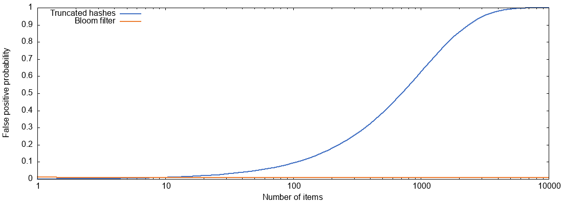
For a Bloom filter, as long as we grow the size of the filter proportionally to the number of items (here we have 10 bits per item), the false positive probability remains pretty much constant at about 0.8%. But truncated hashes of the same size behave much worse, and with more than about 1,000 items the false positive probability exceeds 50%.

The reason for this: with 10-bit truncated hashes there are only 1,024 possible hash values, and if we have 1,000 different items, then most of those 1,024 possible values are already taken. With truncated hashes, if we wanted to keep the false positive probability constant, we would have to use more bits per item as the number of items grows, so the total size of the data structure would grow faster than linearly in the number of items.

Viewing it like this, it is quite remarkable that Bloom filters work as well as they do, using only a constant number of bits per item!

Further details

The Bloom filter false positive formula given above is the one that is commonly quoted, but it’s actually not quite correct. To be precise, it is a lower bound on the exact false positive probability (open access paper).

Out of curiosity I wrote a little Python script that calculates the false positive probability for truncated hashes, Bloom filters using the approximate formula, and Bloom filters using the exact formula. Fortunately, for the parameter values we are interested in, the difference between approximate and exact probability is very small. The gist also contains a Gnuplot script to produce the graph above.

Peter suggested that a Cockoo filter may perform even better than a Bloom filter, but we haven’t looked into that yet. To be honest, the Bloom filter approach already works so well, and it’s so simple, that I’m not sure the added complexity of a more sophisticated data structure would really be worth it.

That’s all for today. Our paper is at arxiv.org/abs/2012.00472. Hope you found this interesting, and please let us know if you end up using the algorithm!